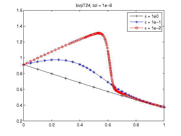
Shock Wave: bvpT24
| shock wave problem: bvpT24 | |
|---|---|
| Contributor: | testset of J.R. Cash |
| Discipline: | fluid dynamics |
| Accession: | 2013 |
Short description:
The problem describes a shock wave in a one dimension nozzle flow. The steady state Navier-Stokes equations generate a second order differential equations that is reduced to a first order system of 2 equations.
Applicable solvers:
all the solvers supported by the Test Set.
Mathematical description:
Consider a shock wave in a one dimension nozzle flow. The steady state Navier-Stokes equations give

where t is the normalized downstream distance from the throat, z is the normalized velocity, A(t) is the area of the nozzle at t , with
![\[z \in \mathbb{R} , \;\;\; t\in [0,1]. \]](https://archimede.uniba.it/~bvpsolvers/testsetbvpsolvers/wp-content/ql-cache/quicklatex.com-9e2eabdf976e8e59a9c27ba612d7fb64_l3.png "Rendered by QuickLaTeX.com")
We write this problem in first order form by defining  and
and  , yielding a system of differential equations of the form

where

with
![\[ (y_1,y_2)^T \in \mathbb{R}^{2} , \;\;\; t \in [0,1]. \]](https://archimede.uniba.it/~bvpsolvers/testsetbvpsolvers/wp-content/ql-cache/quicklatex.com-93b3ab44eea2851df3be738dfccac0d5_l3.png "Rendered by QuickLaTeX.com")
The boundary conditions are obtained from

Given its simple appearence, the BVP turns out to be a surprisingly difficult numerically. An  shock develops, whose location depends on
  .
.
Singular-perturbation-type problems usually require a continuation method to solve them .For this BVP, however, many steps need to be taken.
Download:
- Fortran code: bvpT24.f
- matlab code: bvpT24.m
- R code: first order: bvpT24.R, high order: bvpT24_ho.R